This is number 2 in an irregular series of Experiments That Actually Work [previously].

Using dice to simulate unstable (radioactive) nuclei is a common physics experiment. In the same way that an unstable nucleus has a chance of decaying every second, a die has a chance of decaying every throw. For example: every standard six-sided dice has a one in six (16.67%) chance of decaying each time it’s thrown and every nucleus of niobium-83 has a one in six (actually 16.91%) chance of decaying every second.

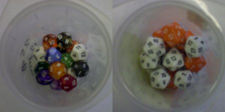
The most significant change made to the “standard” experiment is the use of novel dice. Dungeons and Dragons players use a variety of dice, from the pedestrian 4-sided tetrahedral die (d4) to the more unusual 100-sided (d100) die. We have a complete class set each of 4-sided, 8-sided, 10-sided, 12-sided and 20-sided dice. These dice aren’t particularly expensive, we bought ours in bulk from LegendGames.

The decay constant for each die is the reciprocal of the number of faces, and its mean lifetime is therefore equal to the number of faces. For example, a four-sided die has a decay constant of 0.25 roll⁻¹ and an average lifetime of four rolls. A collection of four-sided dice has a half-life of 2.77 rolls.

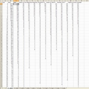
The key to getting good data for this experiment is quantity. When dealing with radioactive samples you’re looking at billions of billions of atoms; so any deviations from the mean are cancelled out, but with dice that unfortunately isn’t possible. I had pupils work individually rather than in pairs and enter all their data into a big spreadsheet. One set of n dice each with s sides should take s + slog_e(n) rolls to fully decay [1]; so fifty 6-sided dice should take about fifty throws, as should twenty-five 12-sided dice; there’s time enough in one lesson to collect a decent dataset.

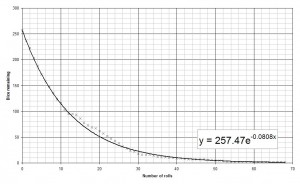
After collecting all the data comes the important graph-plotting stage. Because we’re going to ask Excel to plot a line of best fit that’s exponential in nature, you can’t plot the last data point (dice remaining = 0). Excel won’t allow you to plot an exponential curve if one of the data points is zero.

On the graph I’ve plotted the sum of all the data runs. The most important feature of this graph is the equation of the line of best fit. This is the standard decay equation: N=N₀e^−λt. From the graph above we find that the decay constant is 0.0808 against an expected value of 0.0833, just over 3% less than expected.

As you collect more and more data the value of the decay constant found from the graph gets closer and closer to the correct value – I have a colleague who has a dataset encompassing many years of experiments with 6-sided dice and the value found is within 0.5% of the correct value.

[1] Because (mathematically) exponential decay never actually reaches zero, I’ve calculated this as the number of throws taken to get down to one die remaining, and added the mean lifetime of that die.