Tag Archives: probability

One Million Hats

From the always-excellent Futility Closet, a problem by Paul J. Nahin:

Each of a million people puts his or her hat into a very large box. Each hat has its owner’s name on it. The box is given a good shaking, and then each person, one after another, randomly draws a hat out of the box. What is the probability that at least one person gets their own hat back?

Most people might think that the chance is very, very small, but it’s not. It’s actually more than 60%. How can this be true?

We can view this problem as having only two possible solutions (events): either nobody gets their hat back, or at least one person gets their hat back. The sum of the probabilities of these events must be equal to one and therefore if we can work out the probability that nobody gets their own hat back, then the probability that at least one person does is one minus that.

For each person, there is only a one-in-a-million chance that they have picked their own hat, and thus a 999999 in 1000000 chance that they have not got their own hat.

\Pr \left( \textnormal{one incorrect hat} \right) = \frac{999999}{1000000}

\Pr \left( \textnormal{one million incorrect hats} \right) = \left( \frac{999999}{1000000} \right)^{1000000}

\Pr \left( \textnormal{one million incorrect hats} \right) = 0.368

If the probability of all one million people picking the incorrect hat in 0.368, then via our previous reasoning, the probability of at least one person picking the correct hat is 1-0.368, or 63.2%.

This is a very counterintuitive result, but the wording of the question is key. If we changed the wording to exactly one person getting their hat back then our answer changes dramatically. Starting with our 63.2% chance, we would have to subtract the chance of two people getting their hats back, and of three people getting their hats back, and so on … until we reached the very small chance of one person, and one person only, getting their hat back.
Ranking Ratings

Imagine that you’re trying to rank items that people have either voted for or against. What is the best way to do this?

You could simply take the number of for votes, and subtract the number of against votes. But this doesn’t work if there are a different number of votes for different items: an item with 100 for votes and 50 against votes would be ranked higher than an item with 30 for votes and 1 against vote. You could rank items by their ratio of for votes to against votes, essentially calculating the average score, but this doesn’t work either: an item with just a single for vote (ratio 1.000) would beat an item with 999 for votes and one against vote (ratio 0.999)

The correct method to use in this binomial case is to use the lower bound of Wilson’s score interval:

\mathrm{WSI} = \frac{1}{1 + \frac{1}{n}z^2} \left( \hat p + \frac{1}{2n} \pm z \sqrt{\frac{1}{n}\hat p \left( 1 - \hat p \right) + \frac{1}{4n^2}z^2} \right)

This is a fairly imposing equation, but what’s important is what it does, not how it works.

When ranking items using Wilson’s score interval we are still considering the for-against ratio, but we’re also taking into account the uncertainty created by having a different number of votes for each. For example, consider the following four items:

Item Total Votes Votes For Votes Against Ratio
Item 1 10 5 5 0.5
Item 2 20 10 10 0.5
Item 3 50 25 25 0.5
Item 4 100 50 50 0.5

As you can see, the ratio for each item is the same, but Item 4 received ten times the votes of Item 1 and should therefore be ranked higher.

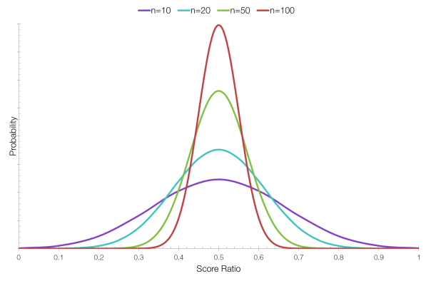
items-graph

In the graph above, each item has the same score ratio, but the curve for Item 4 (n=100) is much sharper around 0.5 because there is less uncertainty about whether it has the “correct” score. An item with only 10 votes might have a “correct” ratio of 0.5, but it’s less likely than for an item with 100 votes.

If we now calculate the lower bound of Wilson’s score interval, we obtain the following results which we can then rank correctly:

Item Total Votes For Against Ratio Wilson SI
Item 1 10 5 5 0.5 0.2366
Item 2 20 10 10 0.5 0.2993
Item 3 50 25 25 0.5 0.3664
Item 4 100 50 50 0.5 0.4038

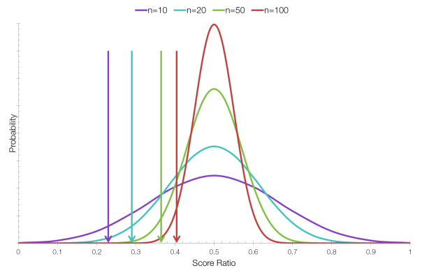
items-graph-indicators

The position of each arrow indicates the lower bound of the Wilson score interval.

In this case we are taking the lower bound of a 95% confidence interval. Taking the lower bound at a confidence interval of 95% means that you are finding, given the data you have, the lowest “correct” score with a probability of 95%. We cannot be 100% sure, so 95% is a good choice – scientists like 95% confidence intervals.

This system could be extended to sites like Amazon that use star rating systems. Currently Amazon calculates a weighted average, which places a product with one ????? rating above a product with one hundred ????? ratings and one ????? rating. A better idea would be to convert the star ratings to for and against votes and use Wilson’s score interval, or a Bayesian model to rank products.

What is “Five Sigma” Data?

or “Why do some experiments take such a long time to run?”

Before you go any further, watch the first minute of this video of Professor Andrei Linde learning from Assistant Professor Chao-Lin Kuo of the BICEP2 collaboration that his life’s work on inflationary theory has been shown by experiment to be correct.

The line we’re interested in is this one from Professor Kuo:

“It’s five sigma at point-two … Five sigma, clear as day, r of point-two”

You can see, from Linde’s reaction and the reaction of his wife, that this is good news.

The “r of point-two” (i.e. r = 0.2) bit is not the important thing here. It refers to the something called the tensor-to-scalar ratio, referred to as r, that measures the differences in the polarisation of the cosmic microwave background radiation caused by gravitational waves (the tensor component) and those caused by density waves (the scalar component).

The bit we’re interested in is the “five sigma” part. Scientific data, particularly in physics and particularly in particle physics and astronomy is often referred to as being “five sigma”, but what does this mean?

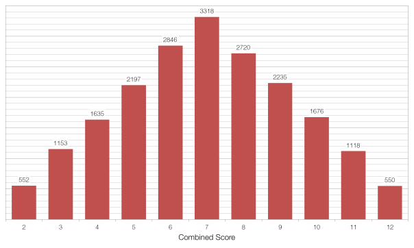
Imagine that we threw two non-biased six-sided dice twenty thousand times, adding the two scores together each time. We would expect to find that seven was the most common value, coming up one-sixth of the time (3333 times) and that two and twelve were the least common values, coming up one thirty-sixth of the time (556 times each). The average value of the two dice would be 7.00, and the standard deviation (the average distance between each value and the average) would be 2.42.

I ran this simulation in Microsoft Excel and obtained the data below. The average was 6.996 and the standard deviation (referred to as sigma or ?) was 2.42. This suggests that there is nothing wrong with my data, as the difference between my average and the expected average was only 0.004, or 0.00385 of a standard deviation, and this is equivalent to a 99.69% chance that our result is not a fluke, but rather just due to the expected random variation.

20000-throws-fair

Now imagine that we have a situation in which we think our dice are “loaded” – they always come up showing a six. If we repeated our 20000 throws with these dice the average value would obviously 12.0, which is out from our expected average by 5.00 or 2.07 standard deviations (2.07?). This would seem to be very good evidence that there is something very seriously wrong with our dice, but a 2.07? result isn’t good enough for physicists. At a confidence level of 2.07? there is still a 1.92%, or 1 in 52, chance that our result is a fluke.

In order to show that our result is definitely not a fluke, we need to collect more data. Throwing the same dice more times won’t help, because the roll of each pair is independent of the previous one, but throwing more dice will help.

If we threw twenty dice the same 20000 times then the expected average total score would be 70, and the standard deviation should be 7.64. If the dice were loaded then the actual average score would be 120, making our result out by 6.55?, which is equivalent to a chance of only 1 in 33.9 billion that our result was a fluke and that actually our dice are fair after all. Another way of thinking about this is that we’d have to carry out our experiment 33.9 billion times for the data we’ve obtained to show up just once by chance.

This is why it takes a very long time to carry out some experiments, like the search for the Higgs Boson or the recent BICEP2 experiment referenced above. When you’re dealing with something far more complex than a loaded die, where the “edge” is very small (BICEP2 looked for fluctuations of the order of one part in one hundred thousand) and there are many, many other variables to consider, it takes a very long time to collect enough data to show that your results are not a fluke.

The “gold standard” in physics is 5?, or a 1 in 3.5 million chance of a fluke, to declare something a discovery (which is why Linde’s wife in the video above blurts out “Discovery?” when hearing the news from Professor Kuo). In the case of the Higgs Boson there were “tantalising hints around 2- to 3-sigma” in November of 2011, but it wasn’t until July 2012 that they broke through the 5? barrier, thus “officially” discovering the Higgs Boson.

Optimal stopping

Imagine a conveyor belt in front of you, on which are placed one hundred various-sized piles of money. You are allowed to stop the belt at any point and take the pile of money in front of you, but you cannot take any pile that has already passed you. Which pile should you take?

There is a mathematical solution to this problem, (sometimes called the Sultan’s Dowry Problem or the Fussy Suitor Problem) which is quite elegant.

  1. Wait until 37% of the piles have gone past you. (The figure of 37% is the reciprocal of e, the base of the natural logarithms.)
  2. Pick the next pile that is better than all the other piles so far.

Here are one hundred randomly-generated piles of money under £100:

£52.33, £80.83, £27.39, £84.75, £63.87, £1.66, £96.82, £76.51, £22.77, £90.94, £24.08, £60.41, £10.38, £95.59, £92.98, £46.80, £85.86, £21.96, £92.22, £29.19, £59.08, £72.22, £45.08, £63.39, £16.38, £71.49, £29.59, £78.62, £30.05, £97.98, £70.95, £3.79, £19.22, £77.52, £1.78, £48.74, £48.71, £35.95, £79.48, £11.50, £47.33, £32.83, £99.19, £3.23, £10.59, £58.22, £21.15, £61.37, £42.78, £25.27, £58.86, £32.82, £91.75, £13.04, £21.76, £72.29, £85.48, £58.81, £8.70, £91.63, £93.30, £23.00, £13.49, £11.67, £95.27, £21.37, £67.27, £90.99, £50.88, £77.22, £9.51, £10.63, £28.23, £63.94, £89.51, £90.12, £68.53, £76.98, £76.83, £92.04, £19.21, £73.82, £71.31, £99.94, £26.96, £86.92, £33.94, £8.25, £13.70, £74.44, £60.08, £11.54, £42.75, £78.67, £41.92, £92.36, £8.25, £92.89, £37.31 and £36.62.

The “best” value from the first thirty-seven piles is £97.98, so you should proceed through the remaining piles until you reach a value greater than this. This means stopping at the 43rd pile: £99.19.

Looking at the data, this strategy doesn’t actually yield the best value – waiting until the 84th pile would yield £99.94, which is slightly more. For large numbers of piles the 37% rule yields the perfect result in only 37% of cases, but this is a greater percentage than any other solution and it usually results in a very good result (i.e. one close to the perfect result).

On the chance of dying in a game of Russian roulette

In a standard game of Russian roulette one bullet is inserted into an otherwise empty “six-shooter” revolver and the cylinder is then spun. Each player then takes turns putting the gun to their head and pulling the trigger until one of them dies.

So if you are forced to play a game of Russian roulette, is there any advantage to going first? Or to going last? Or is it best to play somewhere in the middle?

You might think that as the game progresses your chance of dying increases. In the first round there is a 1 in 6 chance of the bullet being lined up with the barrel; in the second round the chance rises to 1 in 5, all the way through to the final sixth round where the chance is 1 in 1, or certain.

But this is not correct, as you haven’t taken into account the chance that you won’t have to play because someone has already shot themselves in the face. If you multiply the chance of a bullet being in the chamber with the chance of having to play you can calculate the risk of dying in each round.

  • 1st round: 1/6 chance of dying × 6/6 chance of having to play = 1 in 6
  • 2nd round: 1/5 chance of dying × 5/6 chance of having to play = 1 in 6
  • 3rd round: 1/4 chance of dying × 4/6 chance of having to play = 1 in 6
  • 4th round: 1/3 chance of dying × 3/6 chance of having to play = 1 in 6
  • 5th round: 1/2 chance of dying × 2/6 chance of having to play = 1 in 6
  • 6th round: 1/1 chance of dying × 1/6 chance of having to play = 1 in 6

So the answer is no, the turn you take in a game of Russian roulette does not make a difference. Suffice it to say that playing a game of Russian roulette in any way is a Really Bad Idea.