Ranking Ratings

Imagine that you’re trying to rank items that people have either voted for or against. What is the best way to do this?

You could simply take the number of for votes, and subtract the number of against votes. But this doesn’t work if there are a different number of votes for different items: an item with 100 for votes and 50 against votes would be ranked higher than an item with 30 for votes and 1 against vote. You could rank items by their ratio of for votes to against votes, essentially calculating the average score, but this doesn’t work either: an item with just a single for vote (ratio 1.000) would beat an item with 999 for votes and one against vote (ratio 0.999)

The correct method to use in this binomial case is to use the lower bound of Wilson’s score interval:

\mathrm{WSI} = \frac{1}{1 + \frac{1}{n}z^2} \left( \hat p + \frac{1}{2n} \pm z \sqrt{\frac{1}{n}\hat p \left( 1 - \hat p \right) + \frac{1}{4n^2}z^2} \right)

This is a fairly imposing equation, but what’s important is what it does, not how it works.

When ranking items using Wilson’s score interval we are still considering the for-against ratio, but we’re also taking into account the uncertainty created by having a different number of votes for each. For example, consider the following four items:

Item Total Votes Votes For Votes Against Ratio
Item 1 10 5 5 0.5
Item 2 20 10 10 0.5
Item 3 50 25 25 0.5
Item 4 100 50 50 0.5

As you can see, the ratio for each item is the same, but Item 4 received ten times the votes of Item 1 and should therefore be ranked higher.

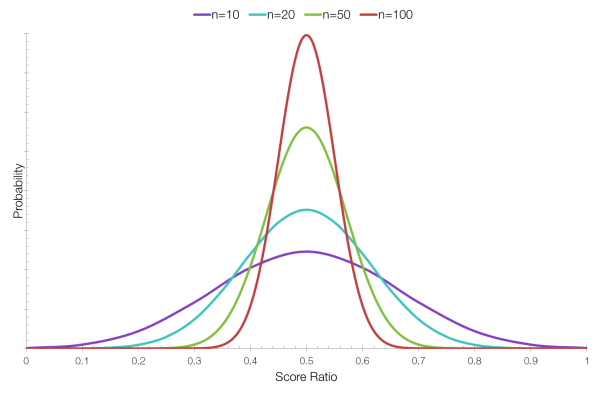
items-graph

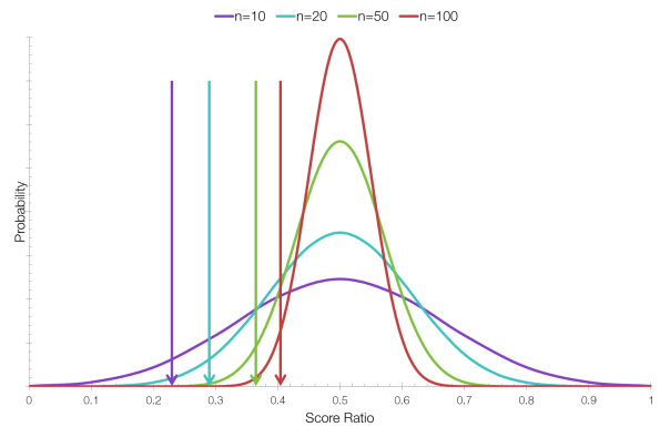
In the graph above, each item has the same score ratio, but the curve for Item 4 (n=100) is much sharper around 0.5 because there is less uncertainty about whether it has the “correct” score. An item with only 10 votes might have a “correct” ratio of 0.5, but it’s less likely than for an item with 100 votes.

If we now calculate the lower bound of Wilson’s score interval, we obtain the following results which we can then rank correctly:

Item Total Votes For Against Ratio Wilson SI
Item 1 10 5 5 0.5 0.2366
Item 2 20 10 10 0.5 0.2993
Item 3 50 25 25 0.5 0.3664
Item 4 100 50 50 0.5 0.4038

items-graph-indicators

The position of each arrow indicates the lower bound of the Wilson score interval.

In this case we are taking the lower bound of a 95% confidence interval. Taking the lower bound at a confidence interval of 95% means that you are finding, given the data you have, the lowest “correct” score with a probability of 95%. We cannot be 100% sure, so 95% is a good choice – scientists like 95% confidence intervals.

This system could be extended to sites like Amazon that use star rating systems. Currently Amazon calculates a weighted average, which places a product with one ????? rating above a product with one hundred ????? ratings and one ????? rating. A better idea would be to convert the star ratings to for and against votes and use Wilson’s score interval, or a Bayesian model to rank products.
UPC Barcodes

This post was inspired by episode 108 of the fantastic 99% Invisible podcast.

UPC barcodes are genuinely ubiquitous. You’ve probably seen a dozen or more UPC barcodes today without even realising or think about it. But how do they work?

A UPC barcode is a graphical representation of a twelve-digit number. What a barcode reader does with that twelve-digit number is the important part from a user’s point of view, but we’re interested in how the barcode reader turns a barcode into that twelve-digit number.

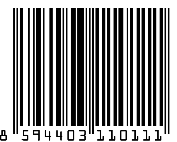
barcode-original

An example UPC barcode. There are thirteen written digits because the last digit is a check digit  which ensures that the code has been entered correctly if it has to be entered by hand.

The first thing to realise is that a barcode is not a pattern of black lines: it is a pattern of black lines and white spaces. A UPC barcode encodes each of the twelve digits in binary, with the black bars representing 1s and the white bars representing 0s. Each digit is represented by seven bits, with each bit represented by a “sub-bar” that is either black or white.

seven-lhs

seven-rhs

The number 7 as represented on the left-hand side (top) and right-hand side (bottom) of a UPC barcode. In binary the representations would be 0111011 and 1000100 respectively.

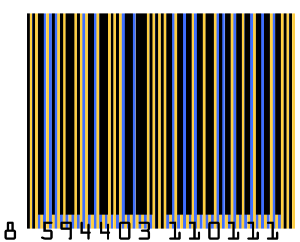
barcode-coloured

The same barcode as above, but with each line of bits (or “pixels”) coloured blue or yellow.

The barcode begins (reading in either direction) with two guide bars that let the barcode scanner know the width of each bit in the barcode, and features another set of guide bars in the centre. The number of black sub-bars for each digit is always odd on the left-hand side of the central guide bars, and even on the right-hand side, which enables a barcode scanner to tell if it is scanning a barcode right-side up or upside-down (see the representations of the number 7 above). The digits start immediately after the guide bar, but as each of the left-hand digits begin with a 0-bit, and each of the right-hand digits ends with a 0-bit, these digits never run into the guide bars or into a following or preceding digit.

With three bits (101) for each of the two guide bars on either side, plus five bits (01010) for the central guide bar, and seven bits for each of the twelve digits, this makes a total of ninety-five bits for the entire barcode. The complete binary representation of the barcode at the top of this post would be:

101 0110111 0110001 0001011 0100011 0100011 0001101 0111101 01010 1100110 1100110 1110010 1100110 1100110 101

(The bits representing the guide bars are shown in bold.)

By reading and decoding this binary series the barcode reader then provides a computer with the twelve digit UPC number, which the computer can then use to control stock, add up prices, etc.

Why Tokyo Looks Different From Space

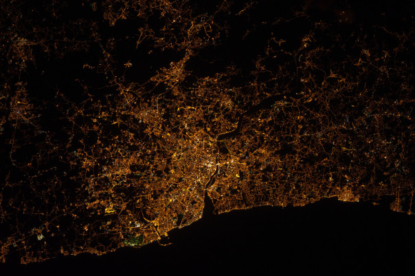
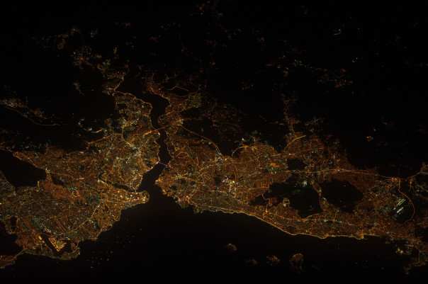
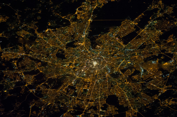
When observed from space at night, most cities look very similar.

porto-night

Porto, Portugal

istanbul-night

Istanbul, Turkey

moscow-night

Moscow, Russia

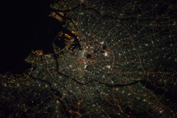
But Tokyo looks very different.

tokyo-night

Unlike most major cities, Tokyo still uses mercury-vapour lamps (which were invented in 1901) rather than sodium-vapour lamps (which were invented in 1920) for its street lighting. The spectra of light emitted by mercury- and sodium-vapour lamps are very different:

sodium-spectrummercury-spectrum

Above: the sodium spectrum; Below: the mercury spectrum.

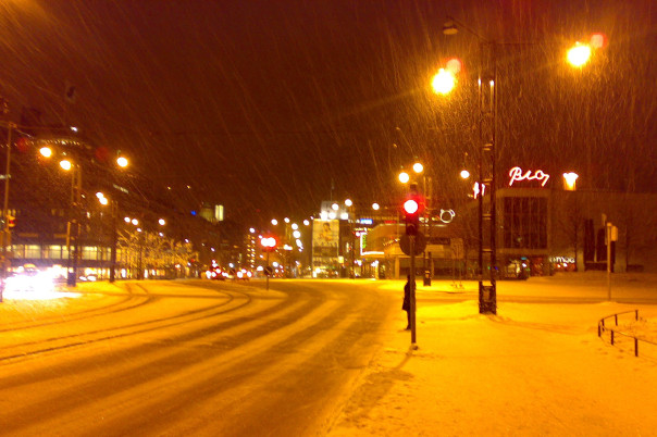
The overall colour of light produced by a sodium-vapour lamp is a bright yellow,* whereas the colour of light produced by a mercury-vapour lamp is a bright turquoise-white.

helsinki-streetSource: naystin

tokyo-streetSource: sinkdd

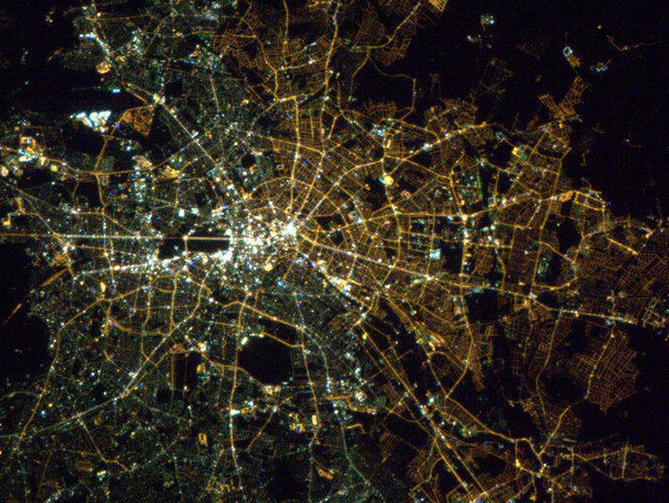
In the photographs above, Helsinki (top) is using sodium-vapour bulbs for its street lighting (though it still has some mercury-vapour lamps it is replacing those), and Tokyo (bottom) is using mercury-vapour bulbs. In Berlin, the division between the old East German and West German parts is still visible from space due to the different types of bulbs used in their streetlamps.

berlin-night

West Germany (on the left of the image) uses mercury-vapour bulbs, and East Germany (on the right) uses sodium-vapour bulbs.

* Light from a sodium-vapour lamp is almost monochromatic, at 589.3?nm. Optical telescope users prefer sodium-vapour light pollution because it is easier to filter out.

Hohmann Transfers

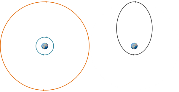
The Hohmann transfer is an orbital manoeuvre used to transfer a satellite between two different circular orbits.

hohmann-orbits
On the left, the two circular orbits between which the transfer will take place. On the right, the elliptical Hohmann transfer orbit.

The orbit of the lower (blue) orbit has the lowest energy (i.e. the specific orbital energy) of the three, the Hohmann transfer orbit has a higher energy than that, and the highest (orange) orbit has the greatest energy of the three.  The gravitational potential and kinetic energies of the initial and final circular orbits are fairly constant, but the gravitational potential and kinetic energies of the Hohmann transfer orbit vary substantially as the orbiting object transfers gravitational potential to kinetic as it approaches Earth and vice versa.

hohmann-transfer

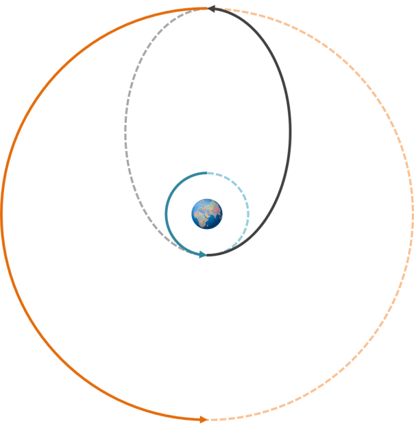
The Hohmann transfer takes place along (half of) an elliptical orbit with one half of the ellipse touching the lower orbit and the other half touching the higher orbit. Two different thruster impulses are used: one to move it onto the elliptical orbit, and then a second one to move it onto the higher orbit. Each time the thruster is fired this increases the kinetic energy of the satellite, which is then transferred to the gravitational potential energy of its new orbit. Because orbits are reversible, moving from a higher orbit to a lower orbit still involves two impulses, but they are in a direction opposite to the motion of the satellite, causing it to decrease in speed and “fall” into the lower orbit.

Sapwood and Heartwood

Until recently, I didn’t realise that there was more than one type of wood inside a tree. The difference was brought to my attention by Earth Science Photo of the Day‘s photo from April 4th.

ebony-sapwood-heartwoodSource: David K. Lynch

The photograph above shows a cross-section through a branch from an ebony tree. The heartwood in the centre is what we traditionally think of as being ebony – almost dark black in colour, whilst the sapwood surrounding it is the more “usual” pale brown colour.

All wood begins as sapwood, and it is sapwood that grows just under the surface of the bark, forming growth rings in the process. Sapwood, as its name suggests, carries sap (transported in tubes called xylem) which the tree uses to store and transport water, sugars (maple syrup is made by reducing xylem sap from maple trees to concentrate the sugars), hormones and nutrients.

In young trees all wood is sapwood, but in older trees, as the tree grows in diameter, less cross-sectional area is required for the transport of sap, and greater structural support is required to keep the tree upright. The sapwood in the centre of the tree dies, forming heartwood, and as the cells die they release chemicals that change the colour of the wood, as well as making the wood stronger and more resistant to attack by insects.

sapwood-comparison

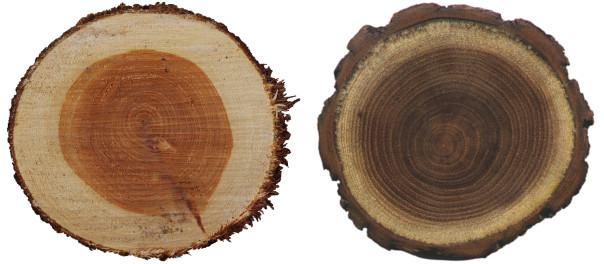
The ratio of sapwood to heartwood depends on how many leaves the tree has and how fast it grows: more leaves and faster growth require more water and therefore more sapwood, and not all trees form any heartwood at all. In the photograph above, a cross-section of a maple tree is on the left and a cross-section of a black locust tree on the right: maple trees have very large leaves, and the black locust trees have small leaves, hence the very obvious difference in their sapwood to heartwood ratios.