Many of you will be familiar with the Beaufort Scale, used to measure wind speed. (Although it’s full name is the Beaufort Wind Force Scale, it does not measure force in the physical sense.) Although the scale is usually taken to relate to open ocean conditions (e.g. Force 6 has been referred to as “Strong Breeze – Long waves begin to form. White foam crests are very frequent. Some airborne spray is present.”) there is an empirical relationship between Beaufort Scale and wind speed:
Where is windspeed and is the 1946 Beaufort Scale.
The Beaufort Scale only officially goes up to Force 12 (“Hurricane Force – Huge waves. Sea is completely white with foam and spray. Air is filled with driving spray, greatly reducing visibility.”) but it could be (and has been) applied to hurricanes (normally measured on the Saffir-Simpson Scale), or tornadoes (normally measured on the Enhanced Fujita Scale). Hurricane Felix, a Category 5 hurricane that struck Nicaragua and Honduras in 2007 had a peak wind speed of 175 mph, equivalent to a Beaufort Scale of 20.7; and the 318 mph wind speed measured by Doppler radar during the Moore Tornado of 1999 would be equivalent to a Beaufort Scale of 30.7.
or “Why do some experiments take such a long time to run?”
Before you go any further, watch the first minute of this video of Professor Andrei Linde learning from Assistant Professor Chao-Lin Kuo of the BICEP2 collaboration that his life’s work on inflationary theory has been shown by experiment to be correct.
The line we’re interested in is this one from Professor Kuo:
“It’s five sigma at point-two … Five sigma, clear as day, r of point-two”
You can see, from Linde’s reaction and the reaction of his wife, that this is good news.
The “r of point-two” (i.e. r = 0.2) bit is not the important thing here. It refers to the something called the tensor-to-scalar ratio, referred to as r, that measures the differences in the polarisation of the cosmic microwave background radiation caused by gravitational waves (the tensor component) and those caused by density waves (the scalar component).
The bit we’re interested in is the “five sigma” part. Scientific data, particularly in physics and particularly in particle physics and astronomy is often referred to as being “five sigma”, but what does this mean?
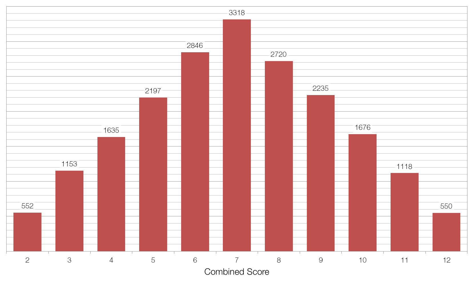
Imagine that we threw two non-biased six-sided dice twenty thousand times, adding the two scores together each time. We would expect to find that seven was the most common value, coming up one-sixth of the time (3333 times) and that two and twelve were the least common values, coming up one thirty-sixth of the time (556 times each). The average value of the two dice would be 7.00, and the standard deviation (the average distance between each value and the average) would be 2.42.
I ran this simulation in Microsoft Excel and obtained the data below. The average was 6.996 and the standard deviation (referred to as sigma or ?) was 2.42. This suggests that there is nothing wrong with my data, as the difference between my average and the expected average was only 0.004, or 0.00385 of a standard deviation, and this is equivalent to a 99.69% chance that our result is not a fluke, but rather just due to the expected random variation.
Now imagine that we have a situation in which we think our dice are “loaded” – they always come up showing a six. If we repeated our 20000 throws with these dice the average value would obviously 12.0, which is out from our expected average by 5.00 or 2.07 standard deviations (2.07?). This would seem to be very good evidence that there is something very seriously wrong with our dice, but a 2.07? result isn’t good enough for physicists. At a confidence level of 2.07? there is still a 1.92%, or 1 in 52, chance that our result is a fluke.
In order to show that our result is definitely not a fluke, we need to collect more data. Throwing the same dice more times won’t help, because the roll of each pair is independent of the previous one, but throwing more dice will help.
If we threw twenty dice the same 20000 times then the expected average total score would be 70, and the standard deviation should be 7.64. If the dice were loaded then the actual average score would be 120, making our result out by 6.55?, which is equivalent to a chance of only 1 in 33.9 billion that our result was a fluke and that actually our dice are fair after all. Another way of thinking about this is that we’d have to carry out our experiment 33.9 billion times for the data we’ve obtained to show up just once by chance.
This is why it takes a very long time to carry out some experiments, like the search for the Higgs Boson or the recent BICEP2 experiment referenced above. When you’re dealing with something far more complex than a loaded die, where the “edge” is very small (BICEP2 looked for fluctuations of the order of one part in one hundred thousand) and there are many, many other variables to consider, it takes a very long time to collect enough data to show that your results are not a fluke.
The “gold standard” in physics is 5?, or a 1 in 3.5 million chance of a fluke, to declare something a discovery (which is why Linde’s wife in the video above blurts out “Discovery?” when hearing the news from Professor Kuo). In the case of the Higgs Boson there were “tantalising hints around 2- to 3-sigma” in November of 2011, but it wasn’t until July 2012 that they broke through the 5? barrier, thus “officially” discovering the Higgs Boson.
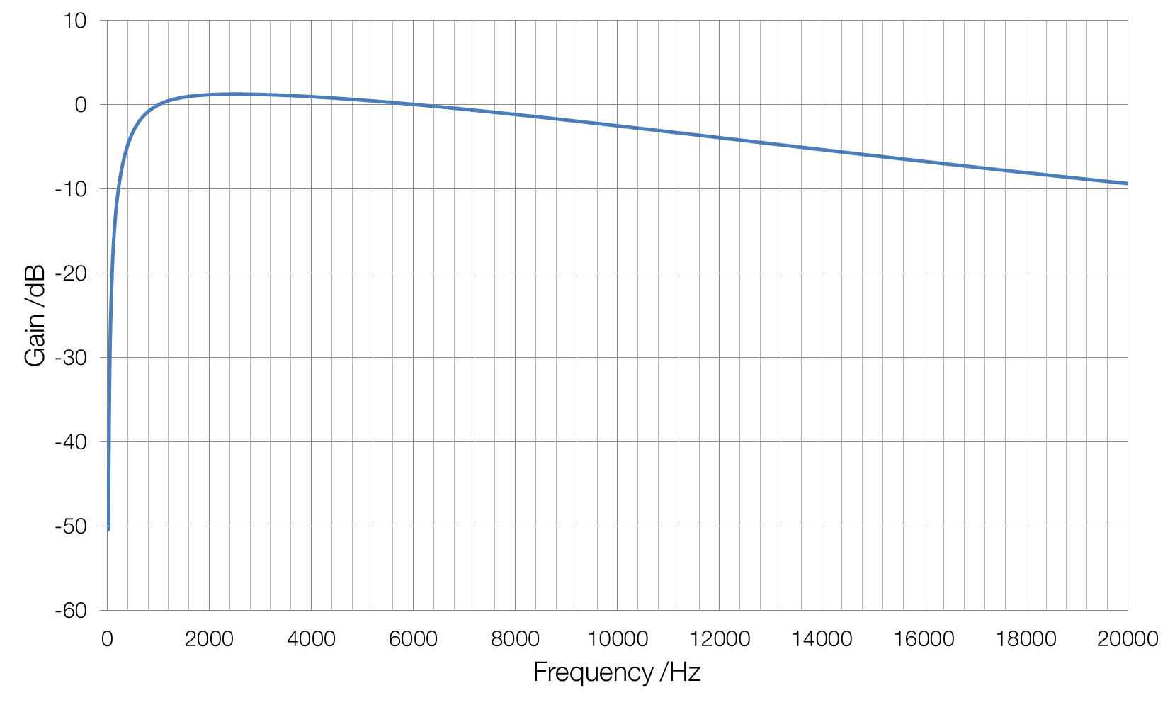
The human ear doesn’t hear equally well at all frequencies. The ear is much less sensitive to low frequencies, below about 1000 Hz, and to high frequencies above about 6000 Hz, and peaks in sensitivity at around 2500 Hz.
A microphone doesn’t have the same issue. This means that after sound is recorded, a filter is applied so that the recorded sound mimics what a human ear would have heard. This filter is called A-weighting, and the volume of sound that is recorded is referred to as dB(A).
dB(A) weighting (linear frequency scale)
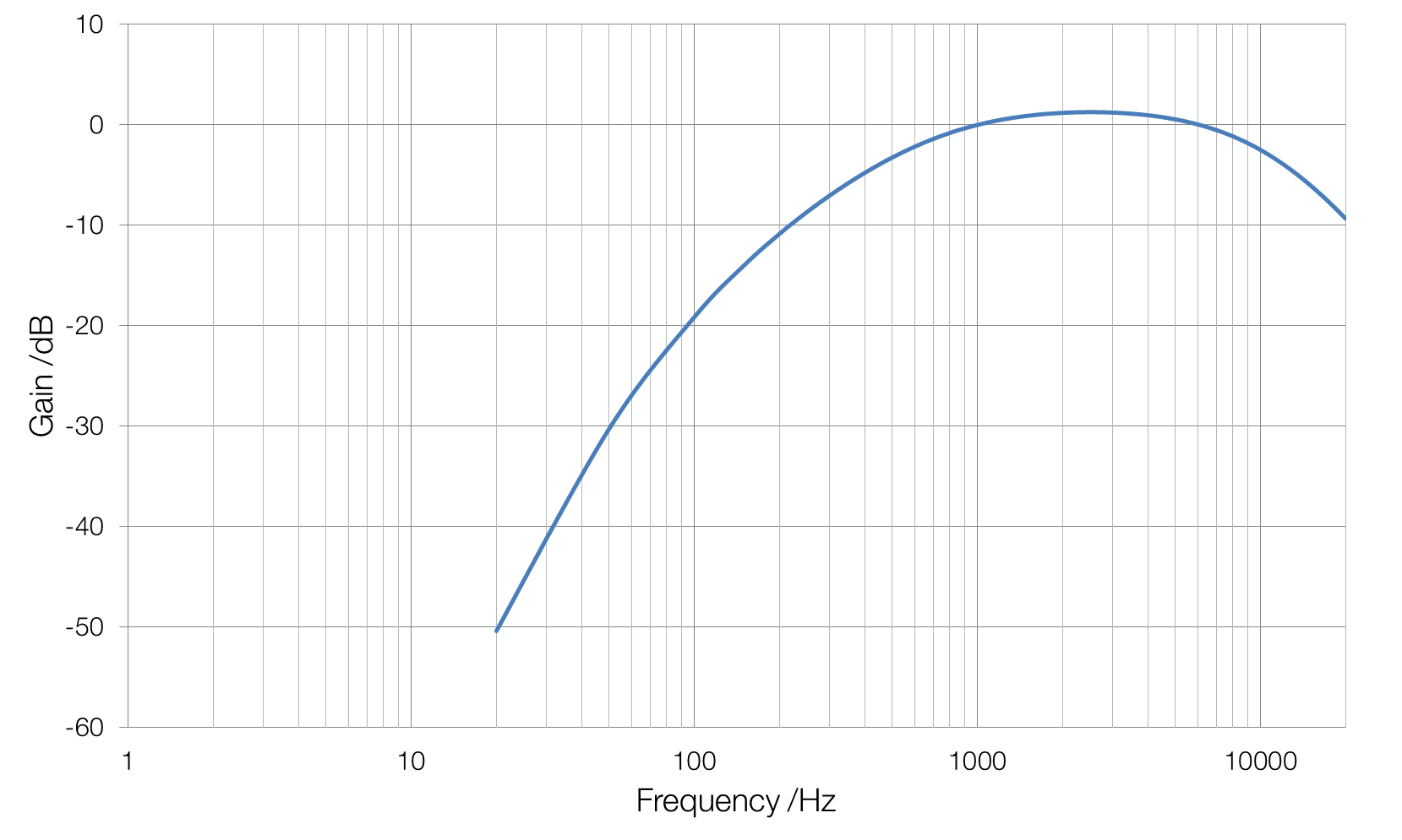
dB(A) weighting (logarithmic frequency scale)
White noise is often taken to be equally loud at all frequencies, but this is not the case: although the sound that is produced is equally loud at all frequencies, this is not what the ear hears. Grey noise is white noise that has been A-weighted so that it is heard to be equally loud at all frequencies.
The Fibonacci Sequence is a very famous sequence of numbers, named after Italian mathematician Leonardo Fibonacci (though the sequence had already been described by Indian mathematicians). Each term in the sequence is composed of the sum of the previous two terms:
F = 1, 1, 2, 3, 5, 8, 13, 21, 34, 55 and so on …
As the sequence grows longer the ratio of each term to the previous term becomes closer and closer to the golden ratio of 1.618 (to four significant figures). This is helpful because the ratio of kilometres to miles is 1.609, which differs by only 0.556 percent.
Therefore, to quickly convert from miles to kilometres you only need to find the value in miles in the Fibonacci sequence and look at the next number in the sequence: 21 miles is 34 kilometres, 34 miles is 55 kilometres and so on. If converting in the other direction, look at the previous term to convert from kilometres to miles.