In computer science, RAID stands for Redundant Array of Independent (or Inexpensive) Disks. A RAID array takes multiple hard drives and treats them as one logical volume – the computer’s BIOS causes your operating system to treat an array of different drives as one single drive.
RAID 0
In RAID 0 data is split across two drives at the block level, in a process called striping. That is, the first part of a file is stored on Drive 1, the second on Drive 2, the third on Drive 1, the fourth on Drive 2, and so on. It offers no redundancy, so if one drive fails the data on both drives is lost, but it does offer improvements in terms of performance. Data can be read and written faster than with one single drive as the first part of a file can be read/written from Drive 1 at the same time as the second part is being read/written from Drive 2.
RAID 0 is most commonly used with two drives of the same size, as the size of the combined volume is limited to twice the size of the smallest drive.
RAID 1
In a RAID 1 setup the data is mirrored on each drive: every block of every file is written identically to each drive (i.e. the data is not striped). This offers the same performance boost as in RAID 0 when reading data, but writing data has to take place on every drive, so is limited by the slowest drive. RAID 1 offers redundancy in that if one drive fails, the data can be recovered from the other still-functioning drives in the array.
RAID 1 is also most commonly used with two drives, but any number of drives can be used in theory. However, there is usually little advantage to this, as it is highly unlikely that more than one drive would fail simultaneously.
RAID 2, RAID 3, RAID 4
RAID 2, RAID 3 and RAID 4 are modifications of RAID 1, but are now obsolete and not commonly used. They stripe data at the bit (RAID 2), byte (RAID 3) or block (RAID 4) level, and also include parity data, which is explained below.
RAID 5
A RAID 5 array must consist of at least three drives. Data is striped across n-1 drives, where n is the number of drives, and parity data (explained below) is stored on the final drive. Thus an array of n identically sized drives yields a combined volume n-1 times the size of each drive, with the striping providing improved performance and the parity data providing redundancy. Parity data is spread out across all drives, which increases performance because during large file writing operations the RAID controller does not have to wait for a dedicated parity drive (as used in RAID 2, RAID 3 and RAID 4) to become available.
For a given file, blocks are stored on different drives and can therefore be read/written simultaneously, which offers some of the speed improvements of RAID 0 and RAID 1 (this also applies if the blocks of different files are located on different drives).
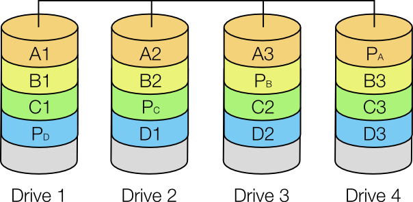
A diagram of a RAID 5 array using four drives.
Parity
For each series of bits parity is calculated by running an exclusive OR (XOR) on the data. An XOR takes individual bits and compares them: a 0 and 0 yields 0, a 0 and 1 or a 1 and 0 yield a 1, and a 1 and 1 yields a 0.
Imagine that we have two blocks of data: 10101010 and 11110000. These two blocks are stored on Drive 1 and Drive 2, and then the two blocks are XORed to yield the parity data which is stored on Drive 3.
Drive 1: 10101010
Drive 2: 11110000
Drive 3: 01011010
Now imagine Drive 2 fails:
Drive 1: 10101010
Drive 2: ????????
Drive 3: 01011010
We know to yield the first parity bit (0) the first bit of Drive 1 (1) must have been XORed with a 1; to yield the second parity bit (1) the bit on Drive 2 must have been a 1, and so on. Thus we can reconstruct the missing data on a new Drive 2. We can also reconstruct missing parity data on a failed drive by simply repeating our original XOR process. However, if two of the three drives fail simultaneously, the data on the two failed drives is lost.
RAID 6
RAID 6 is similar to RAID 5, but distributes parity data across two drives, meaning that it can cope with two drives failing simultaneously and requires a minimum of four drives. RAID 6 is recommended in place of RAID 5 when using high capacity drives in large arrays, as rebuilding an array after a failure puts every other drive in the array under stress, which could cause a second drive to fail.
RAID 10 (aka RAID 1+0)
RAID 10 is a nested array, combining striping and mirroring (and the advantages of both). In the minimal four-drive case, data is striped (RAID 0) between two mirrored (RAID 1) arrays. That is, the first block is mirrored on Drives 1 and 2, and the second block on Drives 3 and 4. A large RAID 10 array can sustain a large number of simultaneous drive failures, providing that no mirror loses all its drives (e.g. in the four-drive example above Drives 1 and 3, 2 and 3, 1 and 4 or 2 and 4 could fail and no data would be lost).
Other nested RAID arrays, such as RAID 50 (combining RAID 5 and RAID 0), or RAID 60 (combining RAID 6 and RAID 0) are also used. You can also use other configurations of drives, such as JBOD (Just a Bunch Of Disks), SPAN/BIG or MAID (Massive Array of Idle Drives).