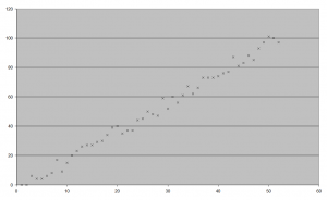
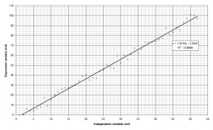
I really hate it when I’m presented with a graph like this one:

It’s instantly recognisable as one created in Microsoft Excel. For some reason the default settings in Excel produce some of the the ugliest graphs I’ve ever seen.

Step 1 – Fix the data points themselves

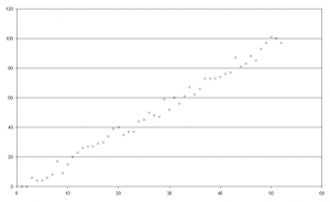
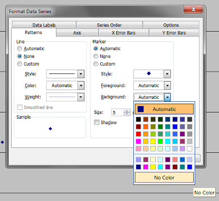
Nobody in their right mind plots data points as little diamonds – we use crosses. Selecting “Format Data Series” enables you to set the background colour to Transparent and the style to a little cross. The colour of the cross is up to you; I tend to stick with traditional black.

Step 2 – Get rid of the background

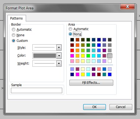
Grey background? Why, Excel, why? Set the ‘Plot Area’ colour to none.

Step  3 – Gridlines

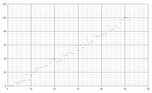
“Standard” graph paper tends to have two sets of lines – thicker major gridlines and thinner minor gridlines. I see no reason why Excel graphs should be any different. Under “Chart Options” there are checkboxes for major/minor gridlines on both the x- and y-axes.

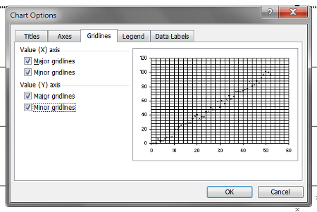
I find that setting the minor gridlines on both axes to a pale grey makes things look nicer. If you’re going to print your graph (or photocopy it) then you’ll want to increase the thickness of the lines too.

Step 4 – The legend

Why Excel puts the legend on the right of the graph I don’t know. Most of the time it’s not needed, and when it is needed it’s far more space-efficient to put it at the top or bottom of the plot area.

Step 5 – Line of best fit

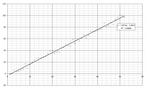
Excel calls lines of best fit ‘Trendlines’ so make sure you add a trendline. Make sure that you choose the right type – exponential for radioactive decay, power for simple pendula, etc.

Step 6 – Axes

Your axes need to be properly labelled.

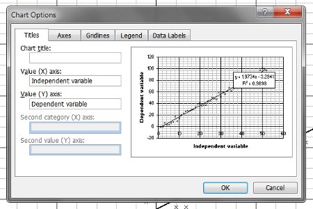
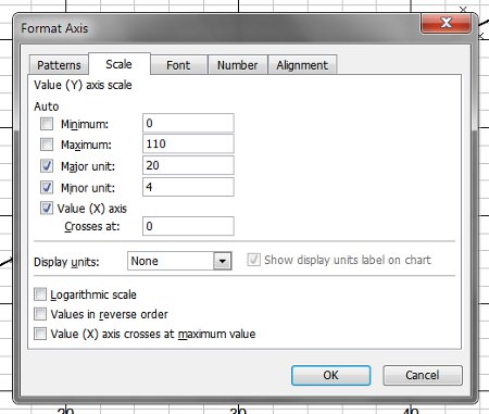
It’s a good idea to adjust the scales as well.

The Finished Product